[Bollinger Bands ①] About Standard Deviation

Problems about Standard Deviation

“In Bollinger Bands, it is described that the probability that price exists between -2σ and +2σ is 95.5%. However, this is incorrect. Explain briefly why.”

John Bollinger, who developed Bollinger Bands, clearly says in his book, “Even if you go above the upper band (+2σ position), that is not a sell signal, and even if you break below the lower band (-2σ position), that is not a buy signal.”

Nevertheless, incorrect buy/sell signals are spreading in Japan. Even though the creator himself denies them.

Obviously, the cause is that people are using technical indicators without properly understanding their definitions and formulas.

Answer

“Because price movements are not normally distributed”

Explanation

Before explaining Bollinger Bands, let's explain standard deviation.

You cannot correctly understand Bollinger Bands without understanding standard deviation.

Standard deviation is a measure of how much data are dispersed.

For example, consider test scores.

Five people’s scores are

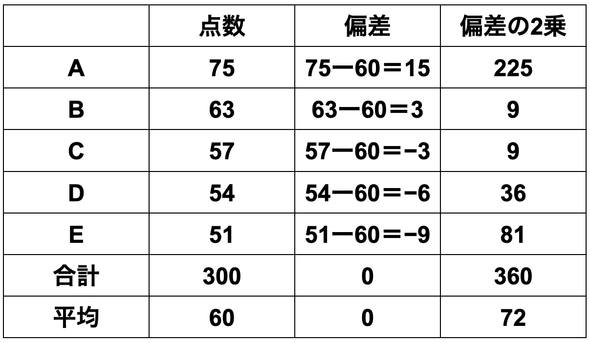
Class 1 [75, 63, 57, 54, 51]

Class 2 [75, 74, 73, 46, 32]

Then

Class 1

① Mean = sum of data ÷ number of data

=(75+63+57+54+51)÷5

=60

② Deviation = each data value − mean

＝[15, 3, -3, -6, -9]

③ Variance = sum of squared deviations ÷ number of data

＝(225+9+9+36+81)÷5

＝72

④ Standard deviation = √72 = 8.48

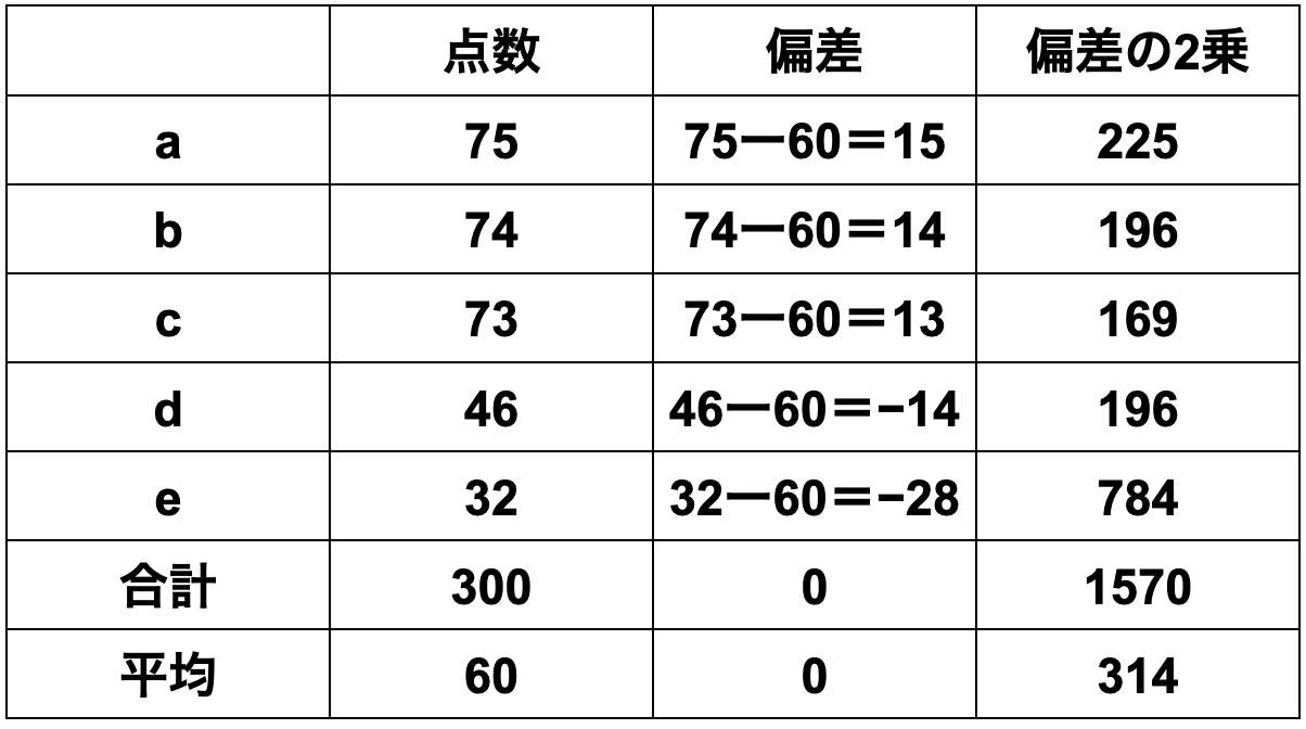
Class 2 is,

① Mean = sum of data ÷ number of data

=(75+74+73+46+32)÷5

=60

② Deviation = each data value − mean

＝[15, 14, 13, -14, -28]

③ Variance = sum of squared deviations ÷ number of data

＝(225+196+169+196+784)÷5

＝314

④ Standard deviation = √314 = 17.72

Because Class 2 has a larger standard deviation, the dispersion is larger.

In university entrance exams, the commonly heard definition of “deviation value” is

Deviation value = 50 + (score − average score) ÷ standard deviation × 10

for this test.

In this test, considering Class 1’s person A and Class 2’s person a, both have

an average score of 60 and a score of 75, with top rank in the class, but their deviation values differ.

Deviation value for Class 1’s person A

＝50 + (75 − 60) ÷ 8.48 × 10

=67.7

Deviation value for Class 2’s person a

＝50 + (75 − 60) ÷ 17.72 × 10

=58.5

Person A has a higher deviation value.

Because the dispersion of data affects the relative position even for the same score.

You might think, “If you want to examine dispersion, you don’t need to square and then take a square root; isn’t it enough to look at deviations from the average?”

That thinking is called the mean absolute deviation. However, it has drawbacks.

For example, suppose there are two classes of 10 students each and both have an average score of 50.

Class 1: 40 points for 5 people, 60 points for 5 people

Class 2: 0 points for 1 person, 100 points for 1 person, 50 points for 8 people

It’s intuitive that Class 2 shows greater dispersion.

But if you sum the deviations from the mean,

Class 1: everyone has a deviation of 10, so total deviation is 100

Class 2: the 0 and 100 point individuals have deviations of 50 each, so total deviation is 100

Thus the mean absolute deviation is the same at 10.

To correctly measure dispersion, you square the deviations; the farther from the mean, the larger the value.

Squaring also has the advantage of eliminating the need to consider plus/minus signs.

Then take the square root to revert the units.

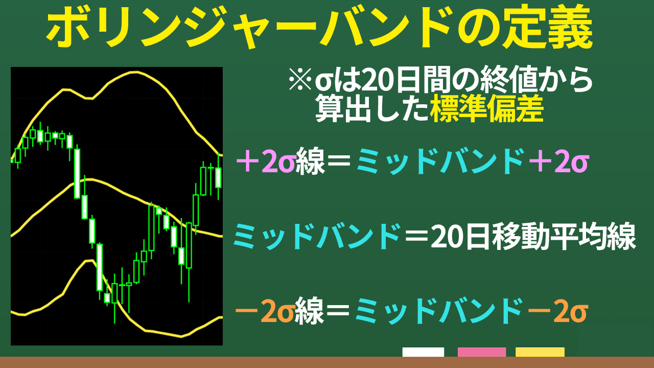
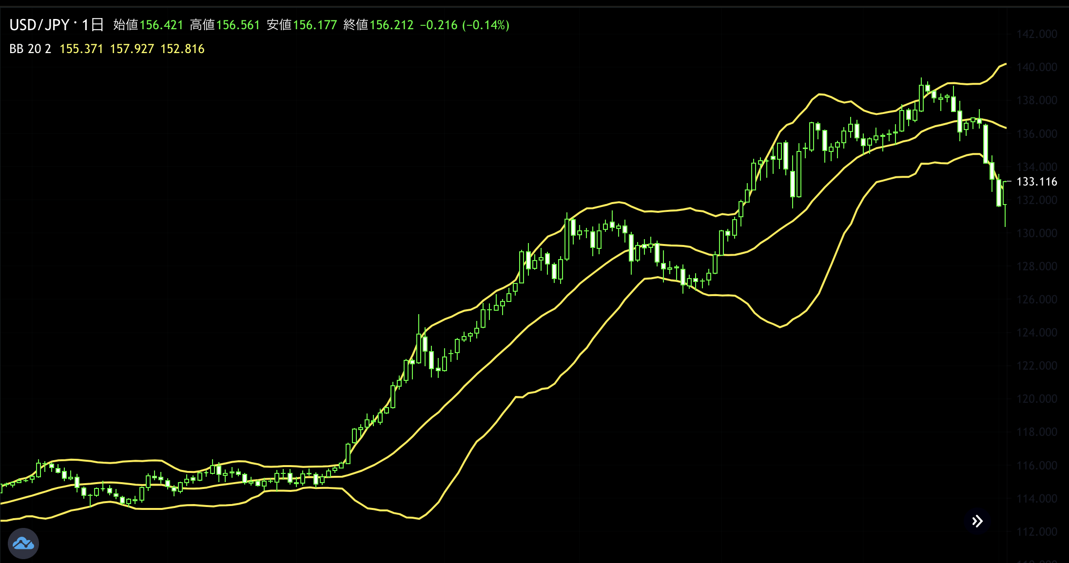
With standard deviation understood, let’s discuss the definition of Bollinger Bands.

If we denote by σ the standard deviation calculated from 20 days of closing prices, centered on the 20-day moving average,

the line plus 2σ is +2σ

the line minus 2σ is −2σ

and these are called.

So what can Bollinger Bands tell us? They indicate volatility.

Back to the test example,

Class 1 standard deviation is 8.48

Class 2 standard deviation is 17.72

Since standard deviation represents data dispersion,

conversely, data are expected to lie within the range around the mean plus/minus the standard deviation.

For Class 1: 60 ± 8.48 = 51.52–68.48 points

For Class 2: 60 ± 17.72 = 42.28–77.72 points

In practice, you can see

Within one standard deviation

Class 1: B, C, D

Class 2: a, b, c, d

Then, what happens if you expand the range to two standard deviations

Class 1: 60 ± 8.48 × 2 = 43.04–76.96

Class 2: 60 ± 17.72 × 2 = 24.56–95.44

With this, all students’ scores in both classes fall within the ±2σ range.

From this idea, the claim that prices stay within the ±2σ range with a probability of 95.5% arises.

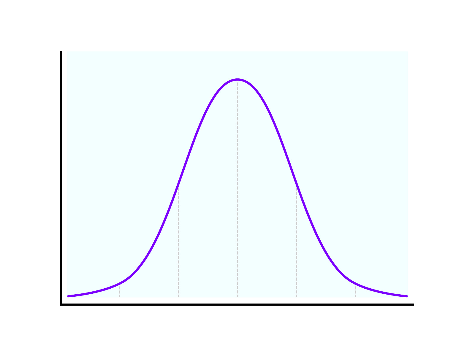
But this holds only when data dispersion follows a normal distribution.

A normal distribution is a probability distribution where the mean, median, and mode are the same and the distribution is symmetric about this axis.

Mean = sum of data values ÷ number of data

Median = the value exactly in the middle when data are arranged from smallest to largest

Mode = the most frequent value in the data

Human height distribution is a good example.

Price movements are not normally distributed, so the statement in the problem is incorrect.

It is not frequent for prices to exceed +2σ and then revert to the center.

However, reaching +2σ and returning to the center does not imply a price increase equals a price decrease!

Did you understand the common mistakes in Bollinger Band explanations on the internet or in books?

The claim that the probability of exceeding ±2σ is less than 5% and thus prices will reverse is incorrect.

Since price movements are skewed, assuming prices will settle within ±2σ is not appropriate.

Next time, we will discuss looking at Bollinger Bands from three perspectives.